pacman::p_load(tidyverse)Hands-on_Exercise1
1.1 Overview
Basic principles and essential components of ggplot2
1.2 Getting started
1.2.2 Importing data
exam_data <- read_csv("data/Exam_data.csv")1.3 Introducing ggplot
1.3.1 R Graphics VS ggplot
hist(exam_data$MATHS)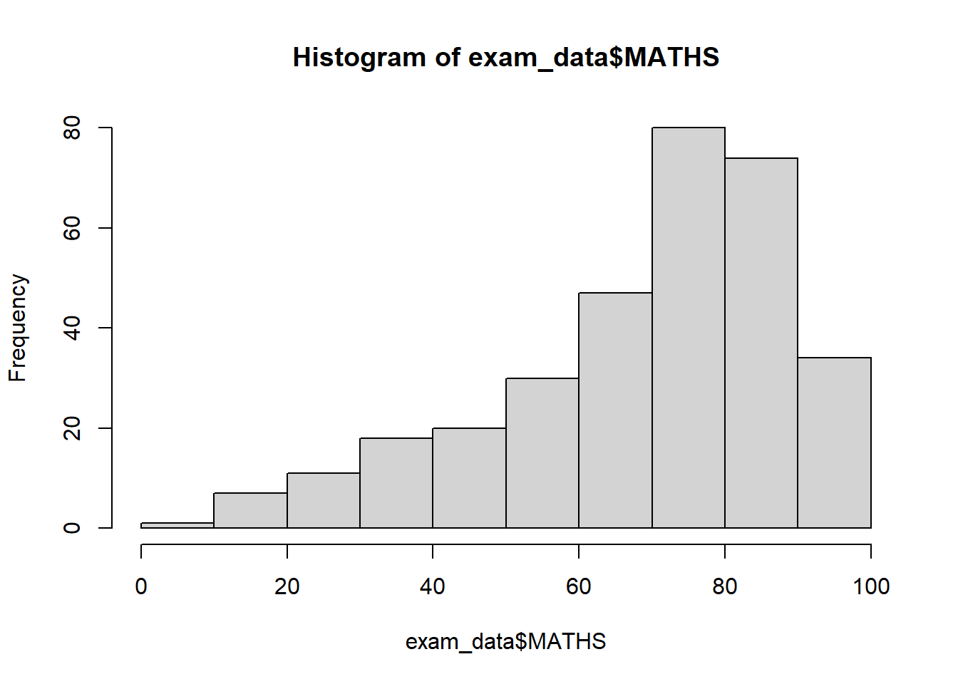
ggplot(data=exam_data, aes(x = MATHS)) +
  geom_histogram(bins=10,
                 boundary = 100,
                 color="black",
                 fill="grey") +
  ggtitle("Distribution of Maths scores")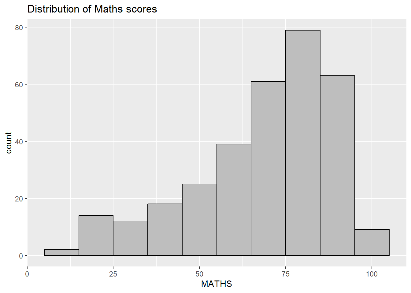
1.4 Grammar of Graphics
1.4.1 A Layered Grammar of Graphics
1.5 Essential Grammatical Elements in ggplot2: data
ggplot(data=exam_data)
1.6 Essential Grammatical Elements in ggplot2: Aesthetic mappings
ggplot(data=exam_data,
       aes(x= MATHS))
1.7 Essential Grammatical Elements in ggplot2: geom 1.7.1 Geometric Objects: geom_bar
ggplot(data=exam_data,
       aes(x=RACE)) +
  geom_bar()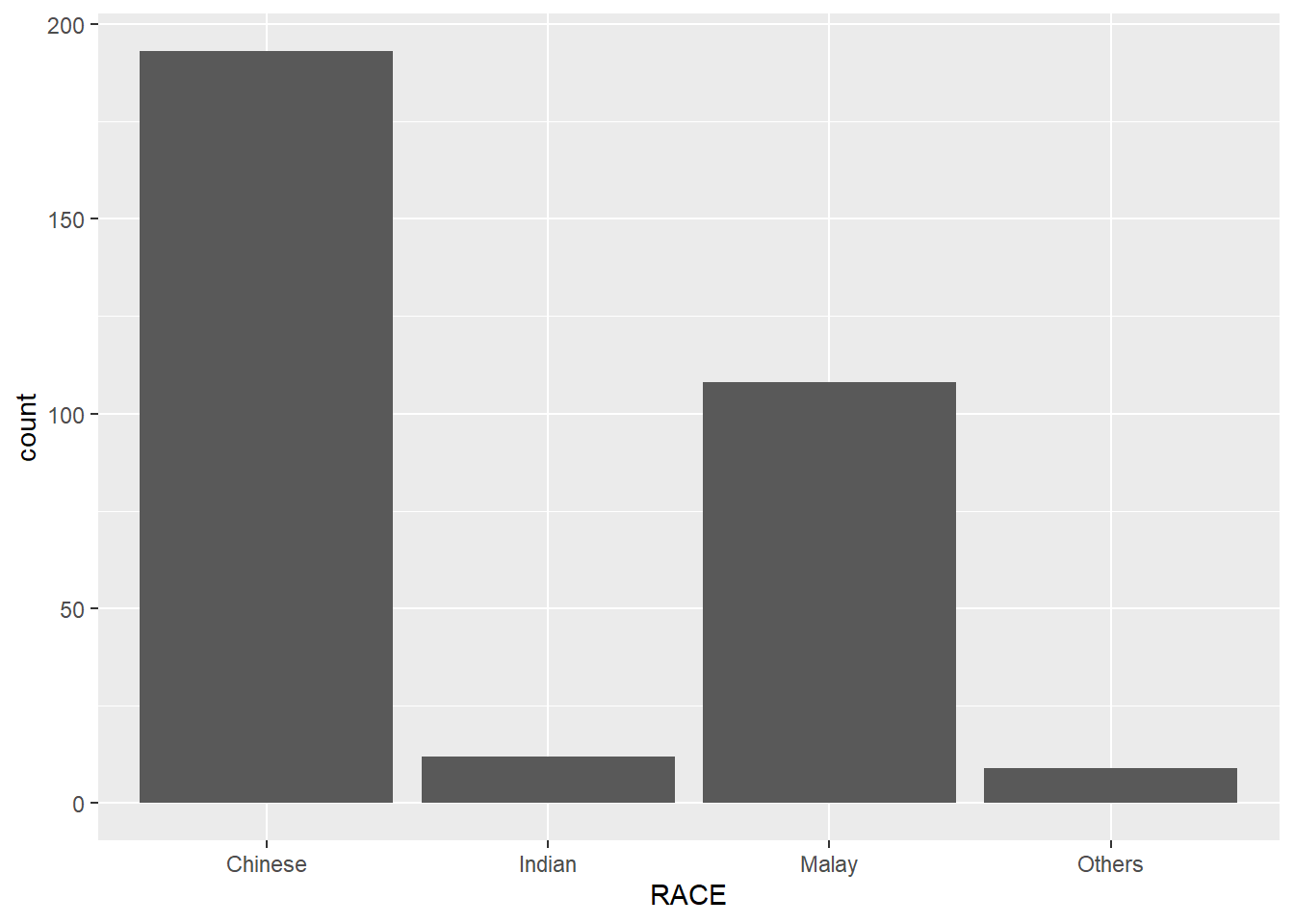
1.7.2 Geometric Objects: geom_dotplot
ggplot(data=exam_data,
       aes(x = MATHS)) +
  geom_dotplot(dotsize = 0.5)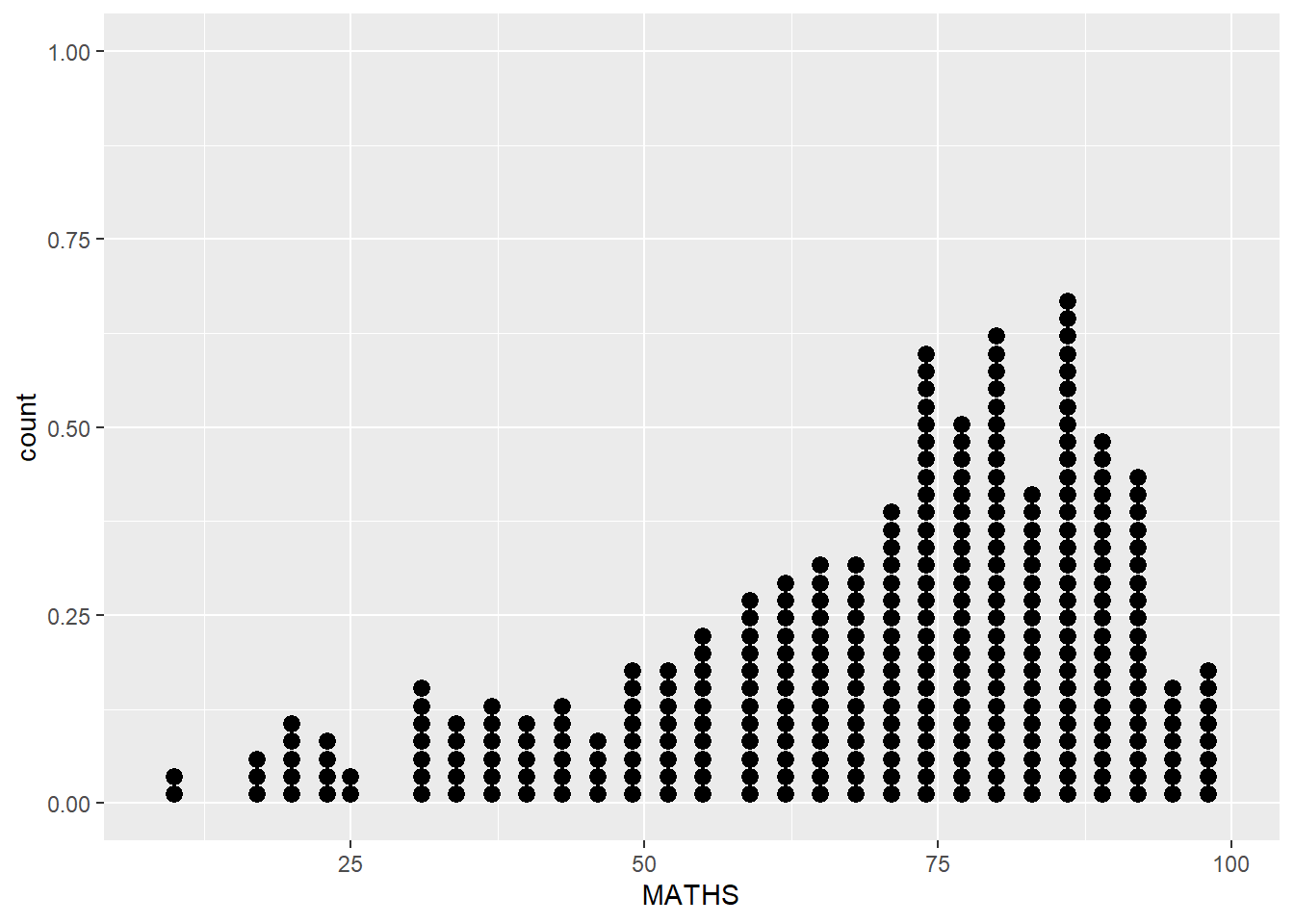
ggplot(data=exam_data,
       aes(x = MATHS)) +
  geom_dotplot(binwidth=2.5,
               dotsize = 0.5) +
  scale_y_continuous(NULL,
breaks = NULL) 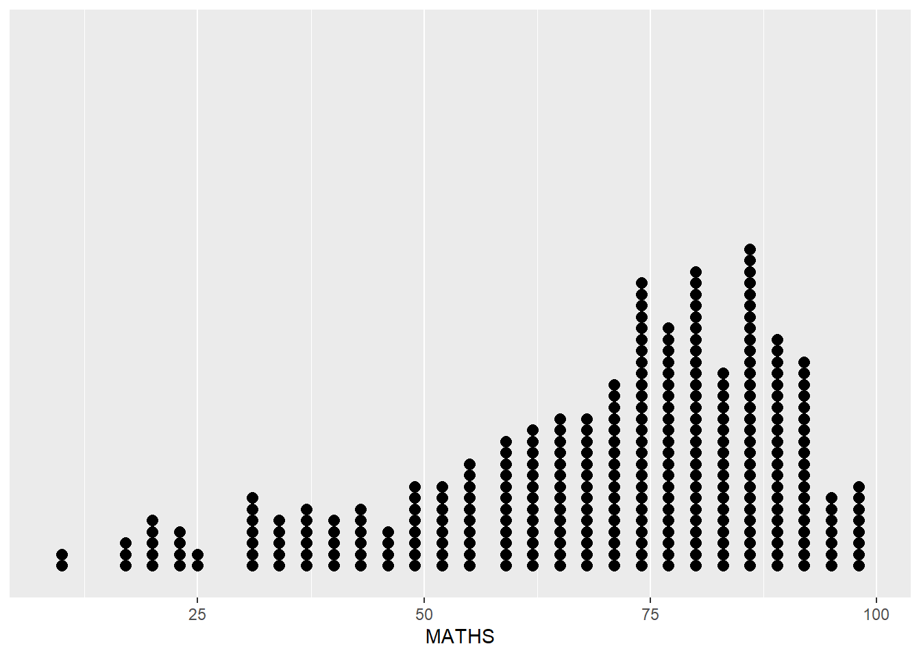
1.7.3 Geometric Objects: geom_histogram()
ggplot(data=exam_data,
       aes(x = MATHS)) +
geom_histogram() 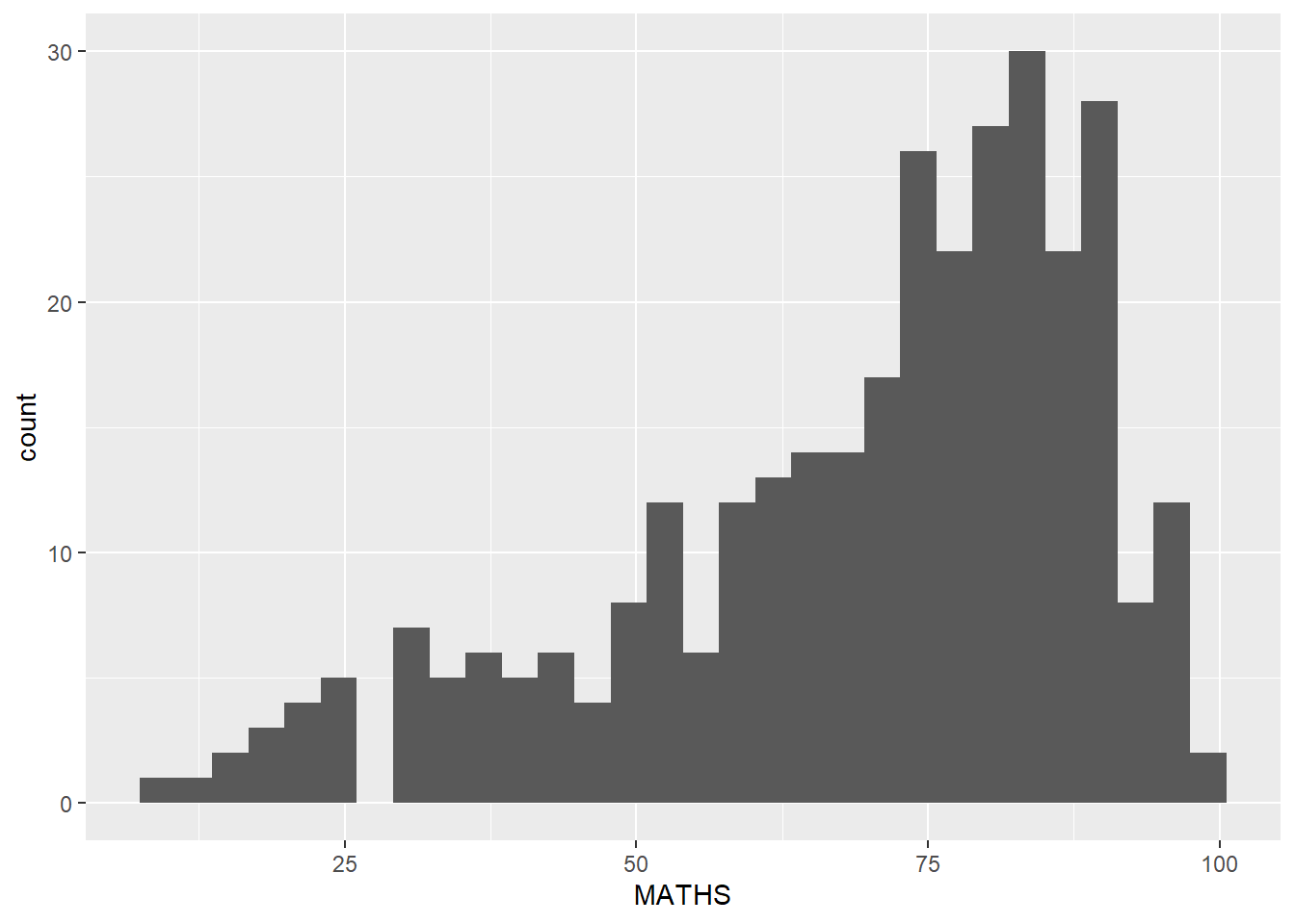
1.7.4 Modifying a geometric object by changing geom()
ggplot(data=exam_data,
       aes(x= MATHS)) +
  geom_histogram(bins=20,
                 color="black",
fill="light blue") 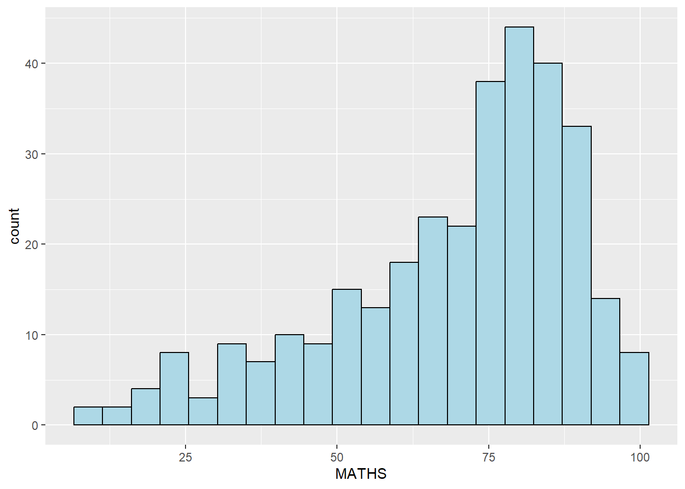
1.7.5 Modifying a geometric object by changing aes()
ggplot(data=exam_data,
       aes(x= MATHS,
           fill = GENDER)) +
  geom_histogram(bins=20,
                 color="grey30")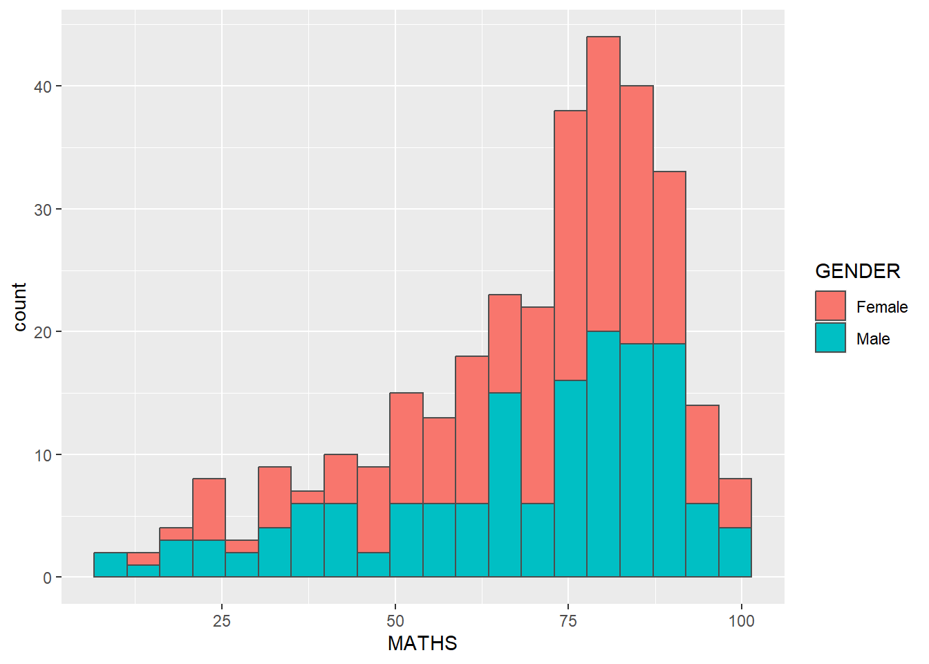
1.7.6 Geometric Objects: geom-density()
ggplot(data=exam_data,
       aes(x = MATHS)) +
geom_density() 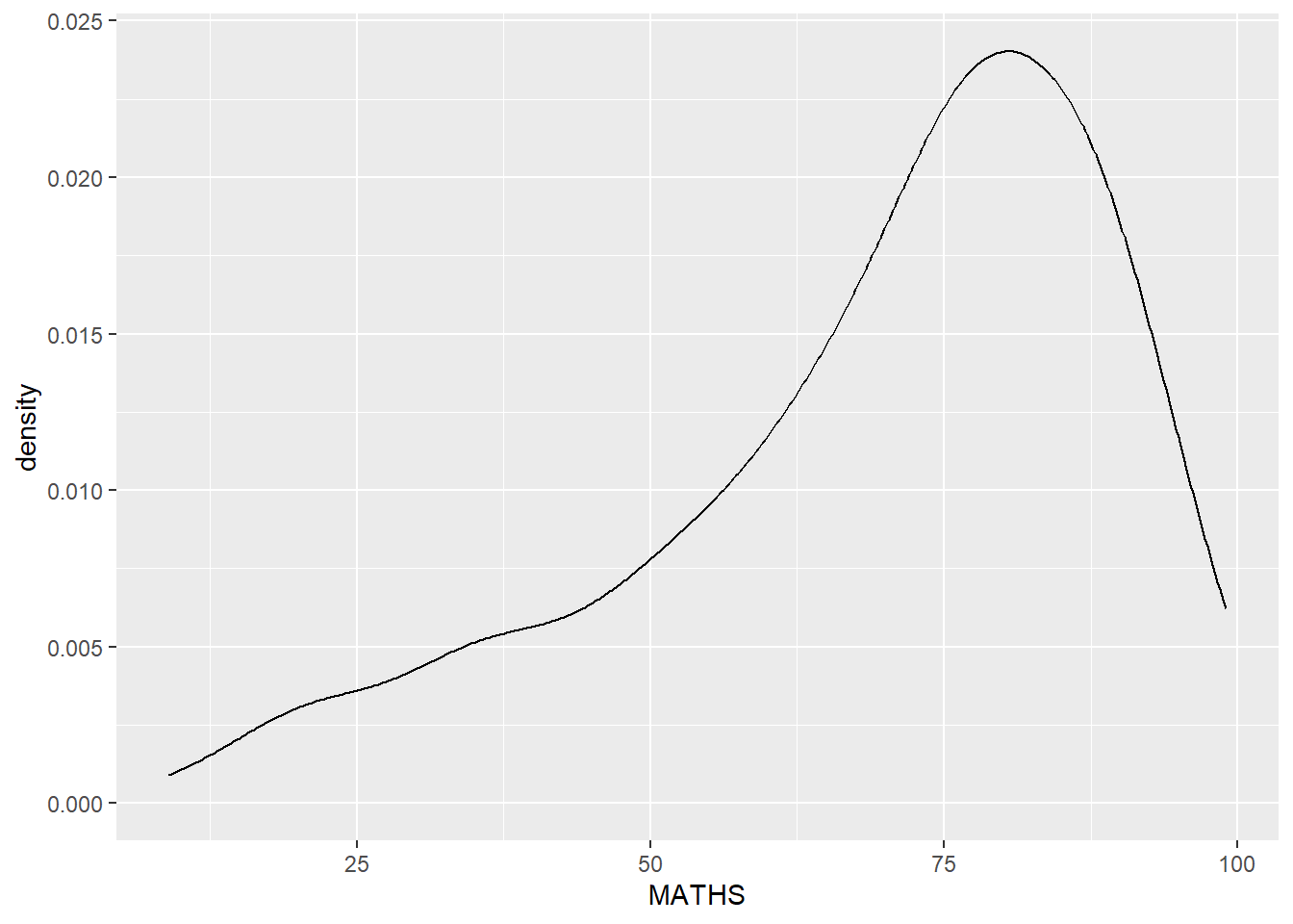
ggplot(data=exam_data,
       aes(x = MATHS,
           colour = GENDER)) +
  geom_density()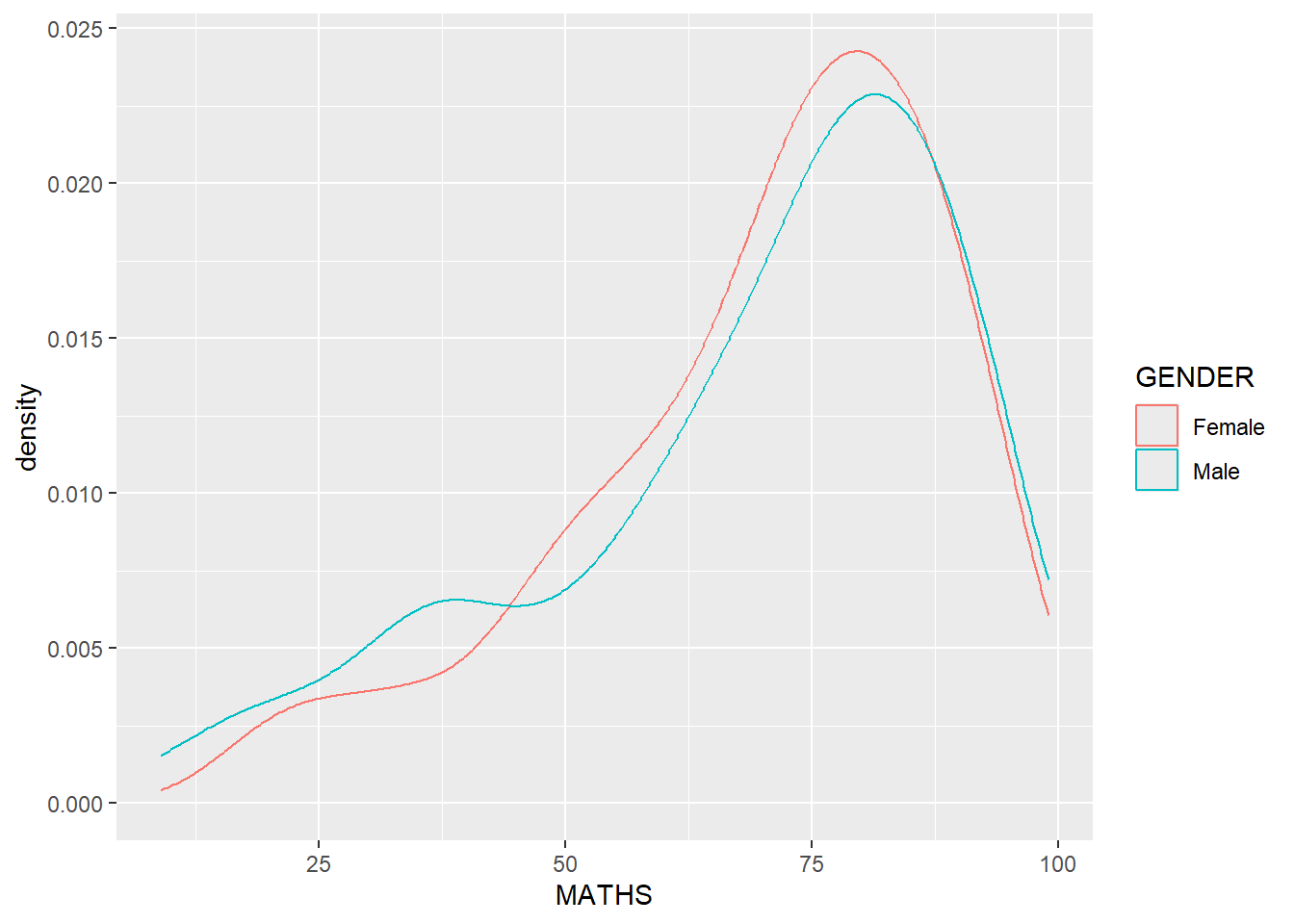
1.7.7 Geometric Objects: geom_boxplot
ggplot(data=exam_data,
       aes(y = MATHS,
           x= GENDER)) +
geom_boxplot() 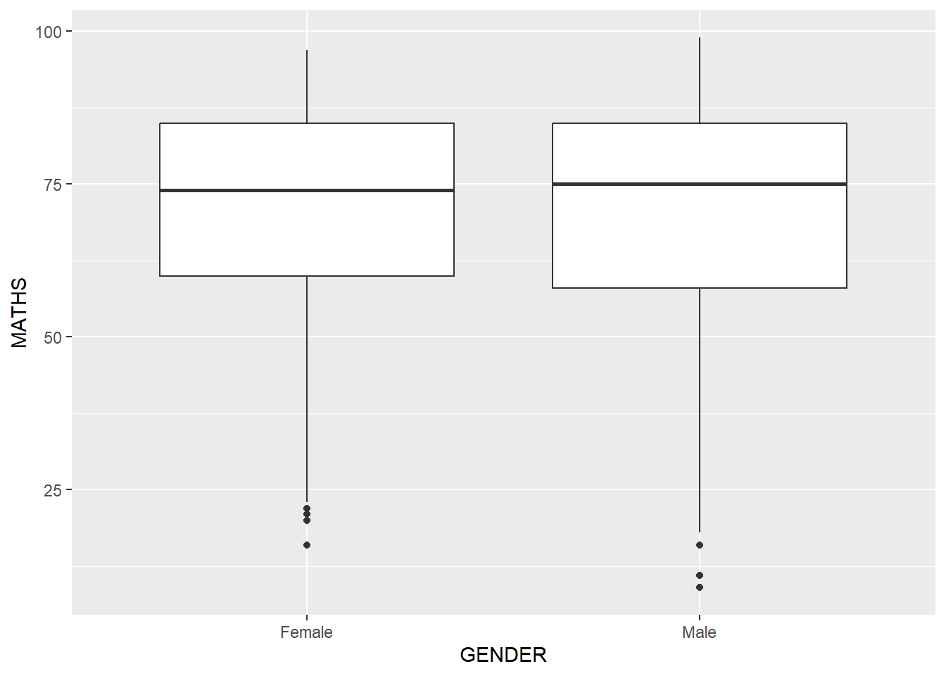
ggplot(data=exam_data,
       aes(y = MATHS,
           x= GENDER)) +
  geom_boxplot(notch=TRUE)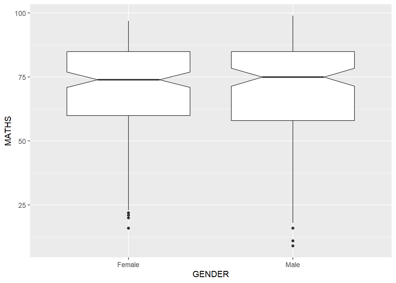
1.7.8 Geometric Objects: geom_violin
ggplot(data=exam_data,
       aes(y = MATHS,
           x= GENDER)) +
  geom_violin()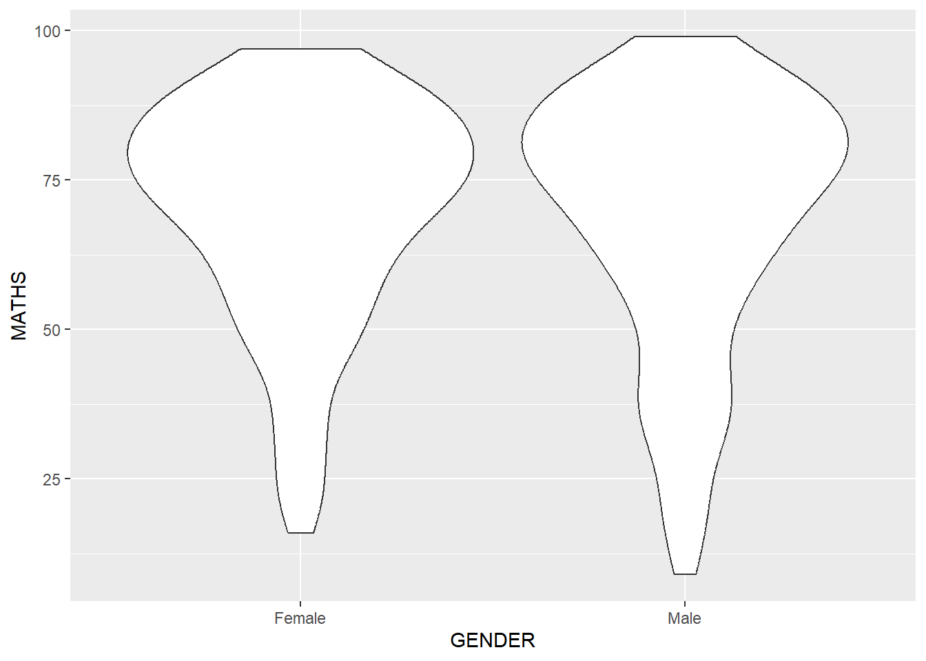
1.7.9 Geometric Objects: geom_point()
ggplot(data=exam_data,
       aes(x= MATHS,
           y=ENGLISH)) +
geom_point() 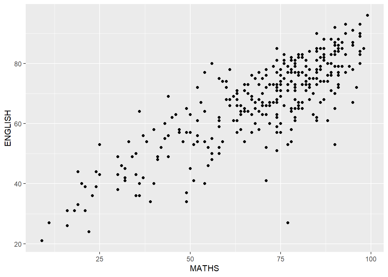
1.7.10 geom objects can be combined
ggplot(data=exam_data,
       aes(y = MATHS,
           x= GENDER)) +
  geom_boxplot() +
  geom_point(position="jitter",
linewidth = 0.5) 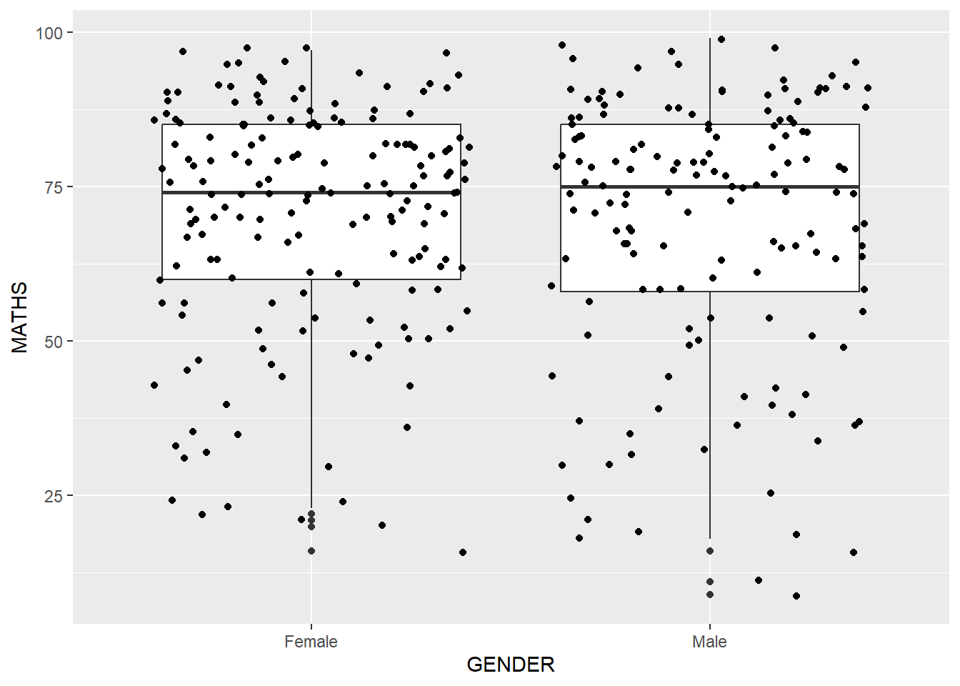
1.8 Essential Grammatical Elements in ggplot2: stat
1.8.1 Working with stat()
ggplot(data=exam_data,
       aes(y = MATHS, x= GENDER)) +
  geom_boxplot()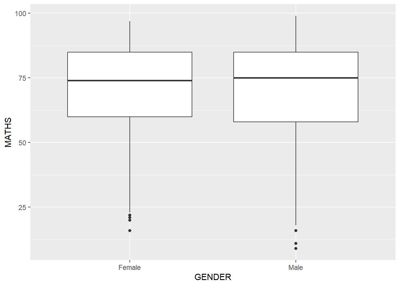
1.8.2 Working with stat - the stat_summary() method
stat_summary() function
ggplot(data=exam_data,
       aes(y = MATHS, x= GENDER)) +
  geom_boxplot()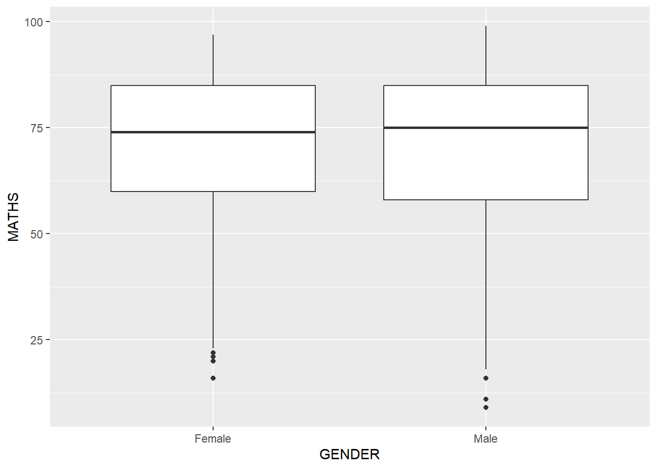
1.8.2 Working with stat - the stat_summary() method stat_summary()
ggplot(data=exam_data,
       aes(y = MATHS, x= GENDER)) +
  geom_boxplot() +
  stat_summary(geom = "point",
               fun = "mean",
               colour ="red",
linewidth=4) 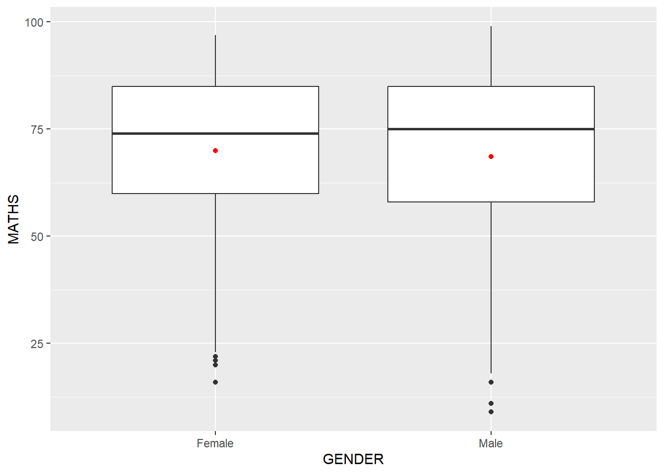
1.8.3 Working with stat - the geom() method
ggplot(data=exam_data,
       aes(y = MATHS, x= GENDER)) +
  geom_boxplot() +
  geom_point(stat="summary",
             fun="mean",
             colour="red",
linewidth=4) 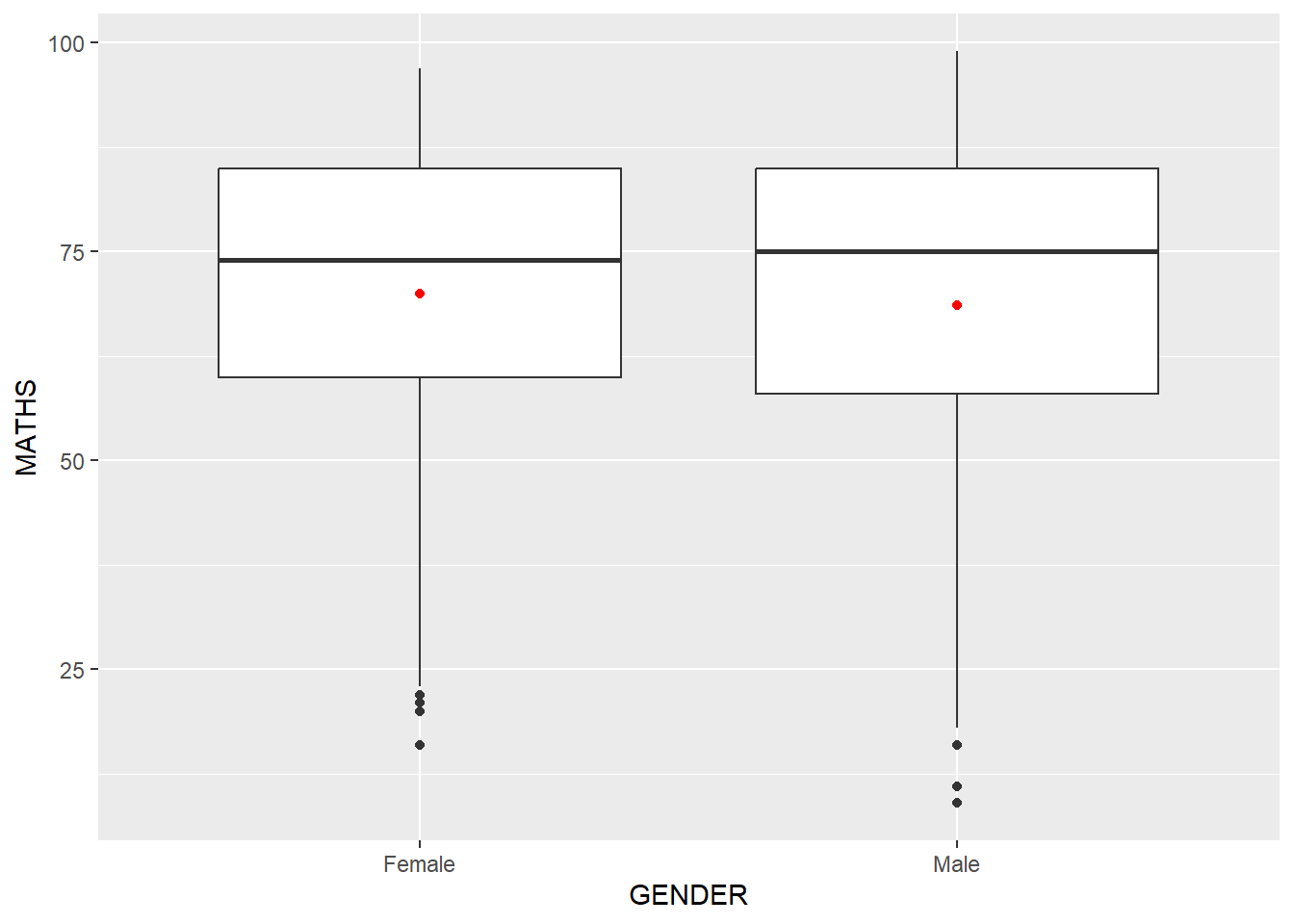
1.8.4 Adding a best fit curve on a scatterplot?
ggplot(data=exam_data,
       aes(x= MATHS, y=ENGLISH)) +
  geom_point() +
  geom_smooth(linewidth=0.5)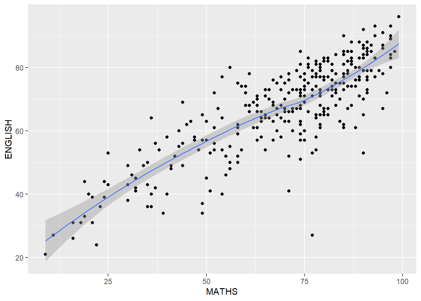
ggplot(data=exam_data,
       aes(x= MATHS,
           y=ENGLISH)) +
  geom_point() +
  geom_smooth(method=lm,
              linewidth=0.5)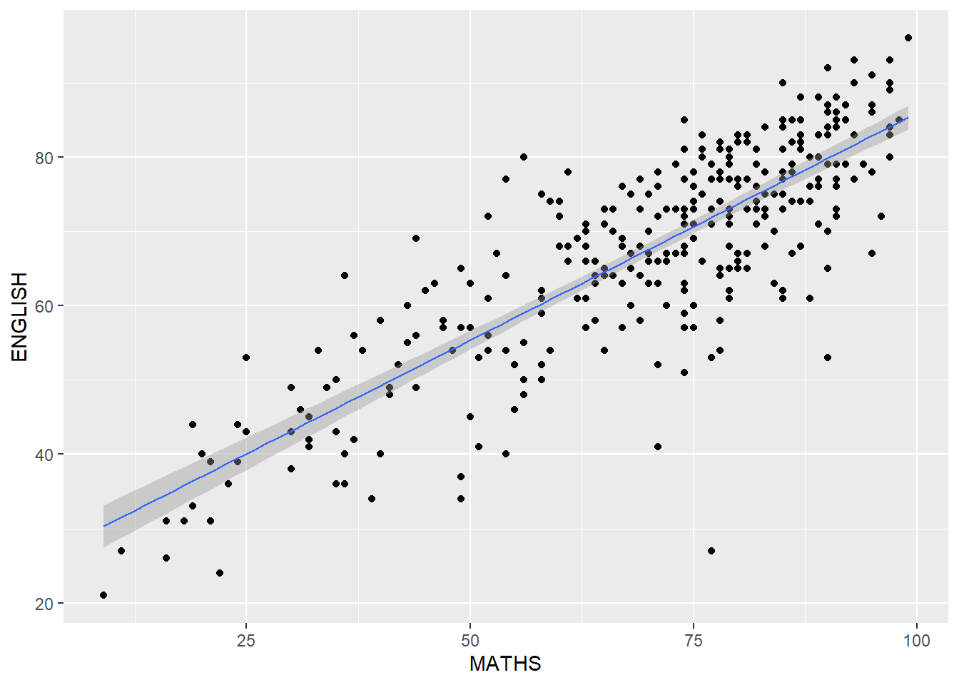
1.9 Essential Grammatical Elements in ggplot2: Facets
1.9.1 Working with facet_wrap()
ggplot(data=exam_data,
       aes(x= MATHS)) +
  geom_histogram(bins=20) +
    facet_wrap(~ CLASS)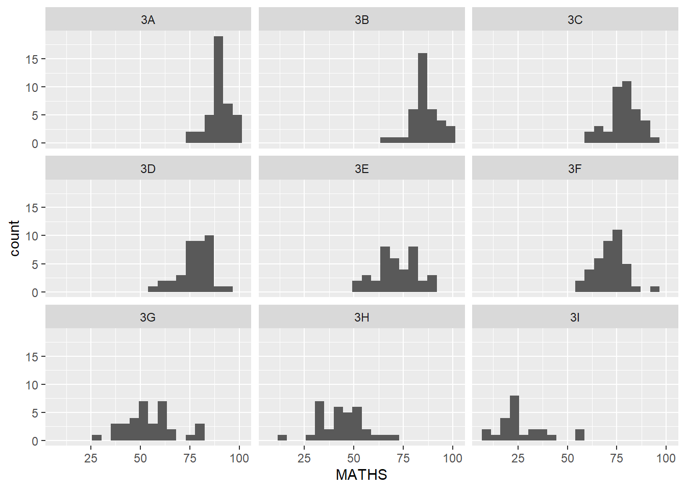
1.9.2 facet_grid() function
ggplot(data=exam_data,
       aes(x= MATHS)) +
  geom_histogram(bins=20) +
    facet_grid(~ CLASS)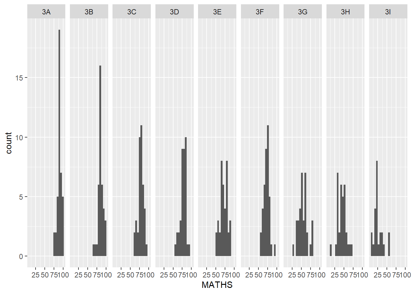
1.10 Essential Grammatical Elements in ggplot2: Coordinates
- [`coord_cartesian()`](https://ggplot2.tidyverse.org/reference/coord_cartesian.html): the default cartesian coordinate systems, where you specify x and y values (e.g. allows you to zoom in or out). - [`coord_flip()`](https://ggplot2.tidyverse.org/reference/coord_flip.html): a cartesian system with the x and y flipped. - [`coord_fixed()`](https://ggplot2.tidyverse.org/reference/coord_fixed.html): a cartesian system with a “fixed” aspect ratio (e.g. 1.78 for a “widescreen” plot). - [`coord_quickmap()`](https://ggplot2.tidyverse.org/reference/coord_map.html): a coordinate system that approximates a good aspect ratio for maps.
1.10.1 Working with Coordinate
ggplot(data=exam_data,
       aes(x=RACE)) +
  geom_bar()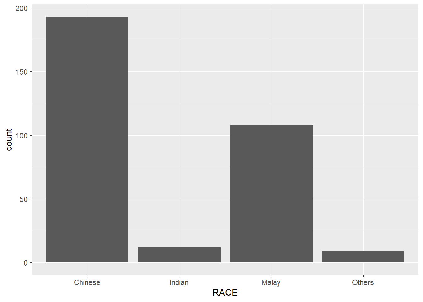
ggplot(data=exam_data,
       aes(x=RACE)) +
  geom_bar() +
  coord_flip()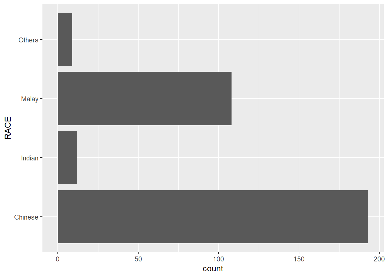
1.10.2 Changing the y- and x-axis range
ggplot(data=exam_data,
       aes(x= MATHS, y=ENGLISH)) +
  geom_point() +
  geom_smooth(method=lm, linewidth=0.5)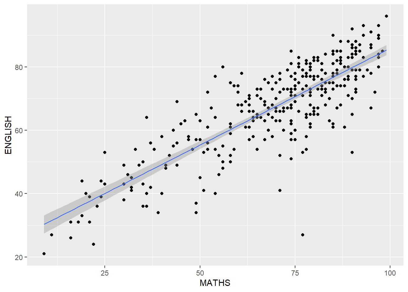
ggplot(data=exam_data,
       aes(x= MATHS, y=ENGLISH)) +
  geom_point() +
  geom_smooth(method=lm,
              linewidth=0.5) +
  coord_cartesian(xlim=c(0,100),
                  ylim=c(0,100))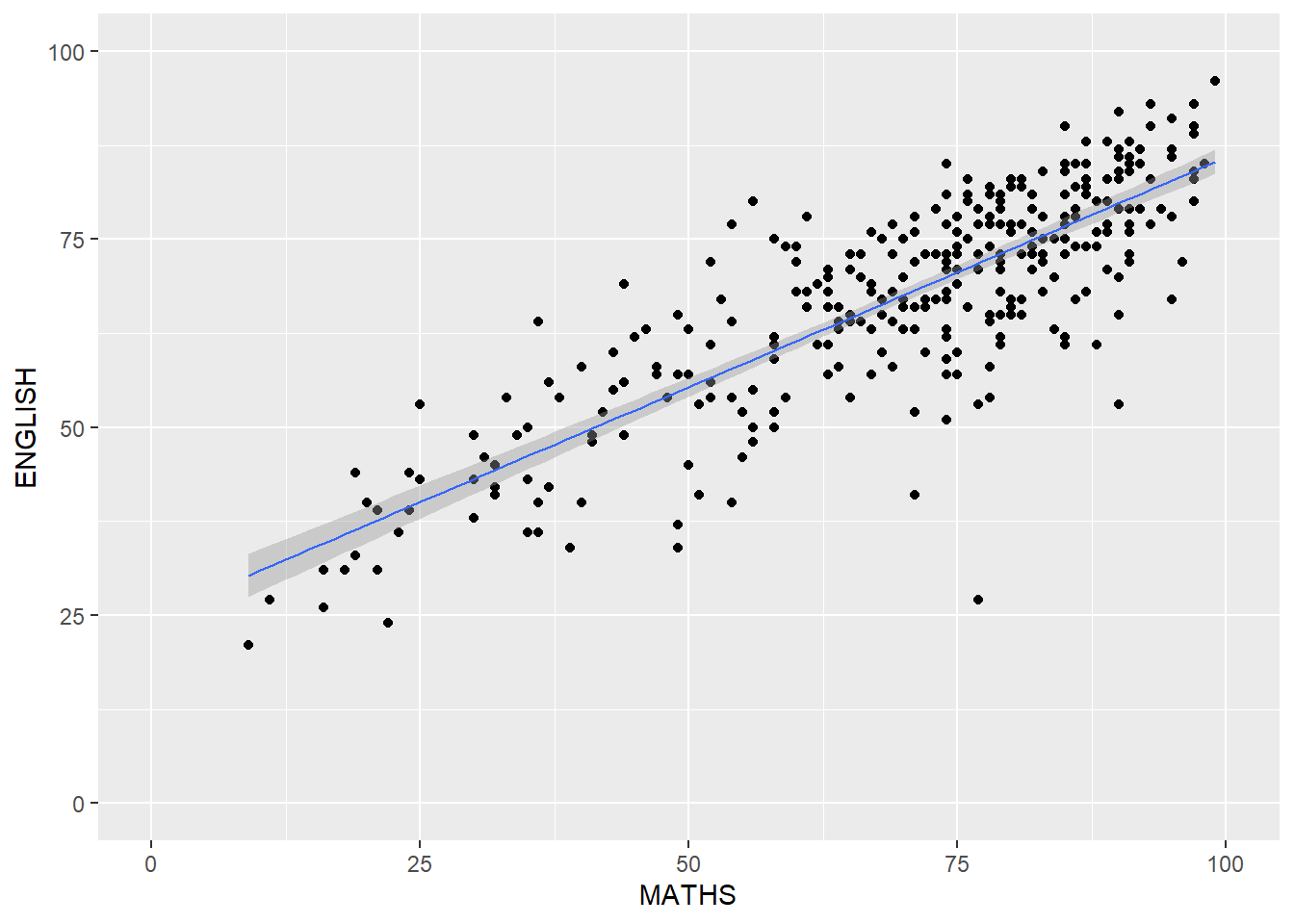
1.11 Essential Grammatical Elements in ggplot2: themes
1.11.1 Working with theme
ggplot(data=exam_data,
       aes(x=RACE)) +
  geom_bar() +
  coord_flip() +
  theme_gray()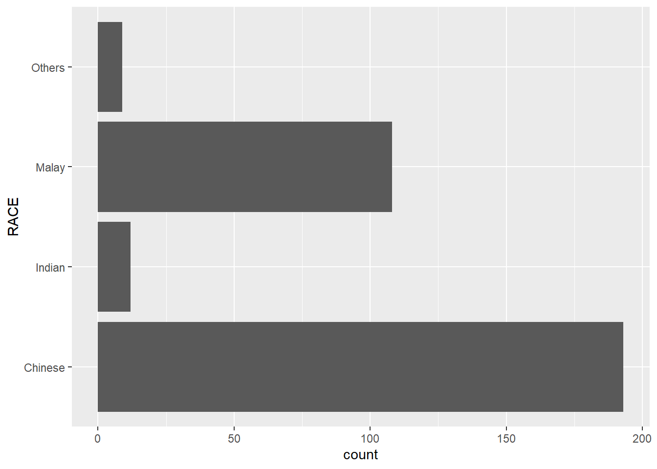
ggplot(data=exam_data,
       aes(x=RACE)) +
  geom_bar() +
  coord_flip() +
  theme_classic()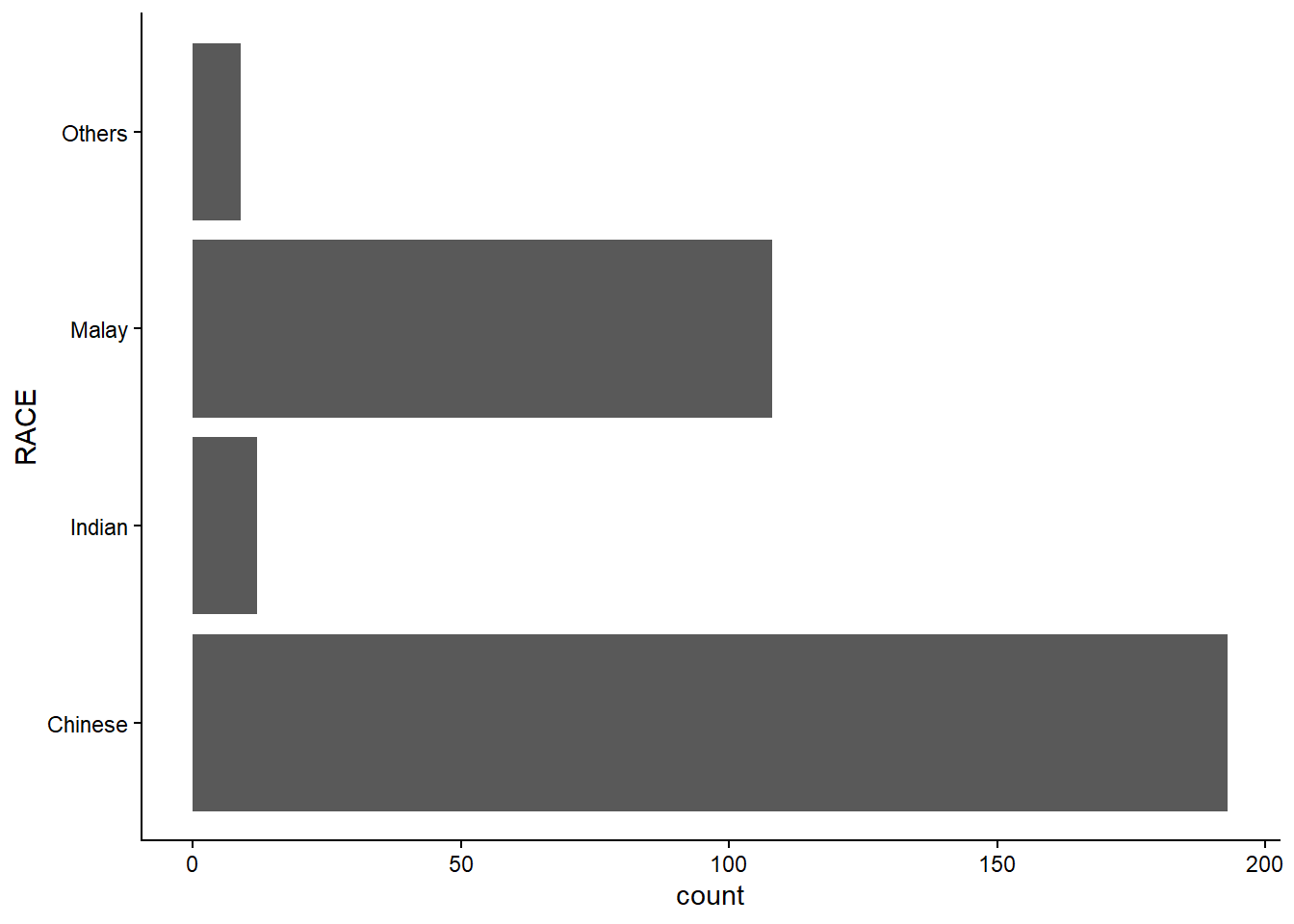
ggplot(data=exam_data,
       aes(x=RACE)) +
  geom_bar() +
  coord_flip() +
  theme_classic()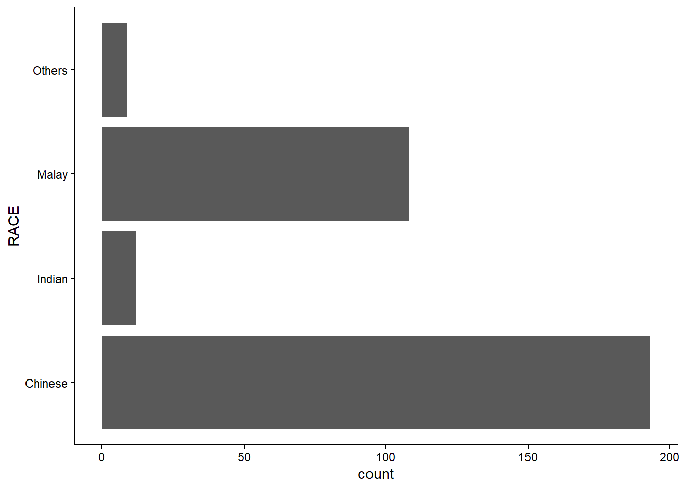
ggplot(data=exam_data,
       aes(x=RACE)) +
  geom_bar() +
  coord_flip() +
  theme_classic()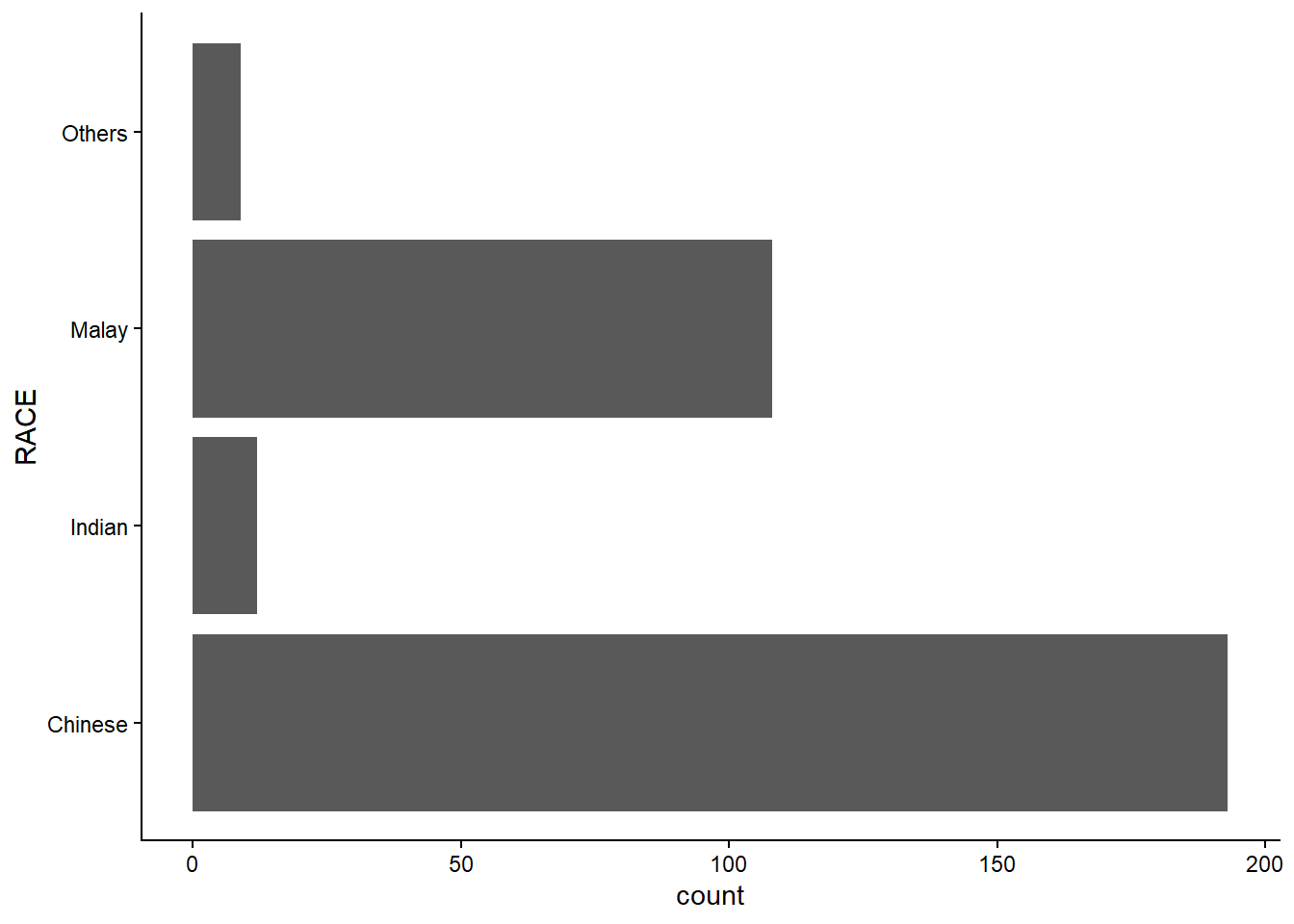
1.12 Reference
Hadley Wickham (2023) ggplot2: Elegant Graphics for Data Analysis. Online 3rd edition.
Winston Chang (2013) R Graphics Cookbook 2nd edition. Online version.
Healy, Kieran (2019) Data Visualization: A practical introduction. Online version